
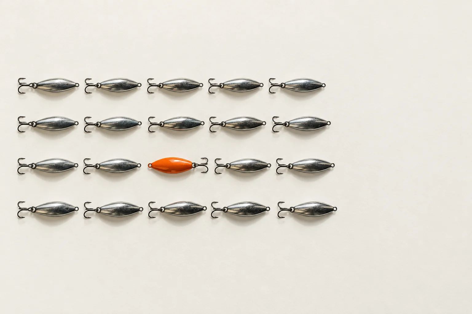
The choice between anomaly detection and supervised classification comes down to two questions: how consistent are your good parts, and how well do you know your defects? Supervised models work when defects are known, recurring and well labeled, and you need to tell them apart. Anomaly detection works when good parts are consistent and defects are rare, varied or not yet seen.
On most production lines, the honest answer is both. A supervised model names the defects you know, and an anomaly model guards against the ones you don’t. The engineering lies in how you set their thresholds, explain their decisions, and turn a new kind of anomaly into a new named class.
Two different questions
A supervised model (a classifier, an object detector or a segmentation network) answers “which of the defects I was taught is this, and where is it?” It learns from labeled examples of every class, including good.
An anomaly detection model answers “how different is this from the good parts I’ve seen?” It trains mostly or entirely on good images. Common approaches compare patches of a new image against a memory of features extracted from good images by a pretrained network (PatchCore is a well-known example), or learn to reconstruct good images and flag regions that reconstruct poorly. Either way, the output is a continuous anomaly score and a map of where the image looks unusual.
The difference sounds academic until a new defect type turns up. A supervised model has to put it into one of the classes it knows, often “good”. An anomaly model only has to notice that it doesn’t look normal.
When supervised classification works
- The defects are known and recurring. You can name them, and enough examples exist or can be collected.
- You need to tell defects apart. Different defects mean different actions, such as rework versus scrap, or routing to a different root-cause owner.
- Good parts vary a lot. Many SKUs, natural materials, printed graphics or textured surfaces make normal variation broad, and an anomaly model would flag too much of it.
- Some defects are tiny. A missing feature a few pixels across may barely move an anomaly score, but a trained detector finds it easily.
When anomaly detection works
- Good parts are consistent. Fixtured parts, controlled lighting, one or a few SKUs.
- Defects are rare or unpredictable. Cracks, contamination and foreign material can take any shape.
- You’re launching something new. A product or line with no defect history yet.
- Defects are hard to create. You can’t produce enough examples without destroying parts.
Its weak spot is that anomalous doesn’t mean defective. A harmless change, such as a new label supplier, a slightly different resin color or a parting line that moves, is anomalous too. Anomaly detection needs controlled imaging and a routine for absorbing acceptable change into its definition of normal.
Data needs compared
| Supervised classification | Anomaly detection | |
|---|---|---|
| Good images | Many, covering normal variation | Many, covering normal variation; this is the training set |
| Defect images | Dozens to hundreds per class, varied | None for training, but real examples are still needed to set and check the threshold |
| Labeling effort | High: every image classed, often with boxes or masks | Low: mainly confirming that training images are good |
| Output | Class, location and confidence | Anomaly score and heat map |
| Fails on | New defect types it was never taught | Normal variation it never saw |
| Typical retraining trigger | A new defect class, or drift | An acceptable process change, or drift |
For a Feasibility Sprint, much smaller sets go a long way, and anomaly models in particular can start from a few dozen good parts. The figures above describe what a production model needs.
One trap is specific to anomaly detection: the training set has to be genuinely good. A few defective parts hidden among thousands of good ones teach the model that those defects are normal, and it will pass them from then on. Curate the good set as carefully as you would curate labels for a classifier, using parts that passed a careful manual inspection rather than everything that came off the line on a given day.
Thresholds and false rejects
Both model types produce a score, and a threshold turns it into a decision. Where you put the threshold is a business decision that looks like a technical one.
For anomaly detection, set the threshold on a held-out set of real good images to meet your false-reject budget, then measure recall on real defects. A hypothetical example: at a threshold that rejects 0.2% of 5,000 good validation parts, the model catches 46 of 50 real defect samples. Lowering the threshold to catch 49 of 50 raises false rejects to 1.1%. Neither setting is “right”. The inspection spec and the cost of an escape decide.
A few practical points:
- Threshold by zone. A visible cosmetic face can carry a stricter threshold than a hidden flange.
- Calibrate supervised confidences. A softmax score of 0.9 is not a 90% probability. Calibrate on validation data (temperature scaling is a simple method) before setting per-class thresholds.
- Use real defects to set thresholds. Synthetic images can help with training, but thresholds must be set and checked against real samples.
- Watch the score distribution. A slow upward creep in anomaly scores on good parts is an early drift warning, often visible weeks before false rejects rise.
- Re-check after change. Thresholds drift with light and material like everything else; see why your inspection model got worse in July.
Explainability: what heat maps can and can’t tell you
Anomaly models produce a heat map as part of their output: the regions that look least like normal. For supervised classifiers, saliency methods such as Grad-CAM show which regions drove the decision, while detectors and segmentation models give boxes or masks directly.
Heat maps earn their keep in three ways. Operators can verify a reject in a second instead of hunting for the defect. Quality engineers can spot a model that is looking at the wrong thing, such as a fixture, a label or the edge of the conveyor. And auditors get a reason attached to every reject image.
They also have limits. Classifier saliency maps are coarse and can mislead, and an anomaly map shows that something is different, not that it is a defect. A heat map supports a person’s judgment; it doesn’t replace looking at the image.
Combining both
In production we usually run both models in parallel on every frame and combine their outputs with explicit rules:
| Supervised model says | Anomaly model says | Decision |
|---|---|---|
| Known defect, confident | Anything | Reject, with the defect’s class |
| Good, confident | Normal | Pass |
| Good, confident | Anomalous | Reject or divert to review as “unknown anomaly” |
| Low confidence | Anomalous | Reject as “unknown anomaly” and queue for labeling |
| Low confidence | Normal | The spec decides: pass, or divert to review |
Running them in parallel rather than as a strict gate matters. Some known defects are too small to move the anomaly score, so a design that only calls the classifier on anomalous frames would let them through. The rule for disagreements, reject or divert, belongs in the inspection spec, not buried in the integrator’s code.
Handling new defect types
The combination shows its real value when something new appears:
- The anomaly model flags parts the classifier can’t name.
- Reviewers work through the “unknown anomaly” queue, with similar images grouped by embedding similarity so recurring patterns stand out.
- When a pattern recurs, a quality engineer names it, adds it to the defect catalogue and sets its limit samples.
- Examples are collected, real ones first, with synthetic augmentation only where real examples are scarce.
- The classifier is retrained with the new class, validated on real data, and the model card is updated.
Until step 5, the anomaly model is what keeps the new defect off the truck.
A short decision guide
- Consistent parts with rare or unknown defects: start with anomaly detection.
- Little or no defect history: anomaly detection now, adding supervised classes as real defects are collected.
- Known defects that need different actions: supervised classification or detection.
- Highly variable good parts: supervised, with careful data collection.
- Anything safety- or recall-critical: both in parallel, with the disagreement rule written down.
Pick the model for the line you have
There is no universally better model, only a better fit for your parts, your defects and your data. Our AI visual inspection systems combine both approaches so new defect types are flagged rather than passed, and our synthetic data and model training work covers building the datasets each model needs.